Omics Data Collection & Preparation
Overview
Teaching: 30 min
Exercises: 30 minQuestions
What is the experimental design for the data set we are using?
How do I naviagate the terminal?
How should I prepare data for analysis?
What are the most common file formats of transcriptomic and genomic data?
What are some databases and software tools I can use to collect omics data?
Objectives
Gain an understanding of the source of our data.
Become familiar with how transcriptomic and genomic data is structured.
Be able to install and use necessary bioinformatics software tools.
Become familiar with best practices in preparing data for analysis.
Gain hands-on experience and develop skills to be able to use BASH to gather omic data for analysis.
Develop BASH scripting skills to efficiently integrate R scripts into a coherent data analysis pipeline.
Study Design & Data Collection
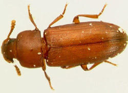
As a first step, we will begin with collecting some data for analysis. In this workshop we will be using data from a study of the effects of ultraviolet (UV) radiation on the larvae of the red flour beetle, titled “Digital gene expression profiling in larvae of Tribolium castaneum at different periods post UV-B exposure”.
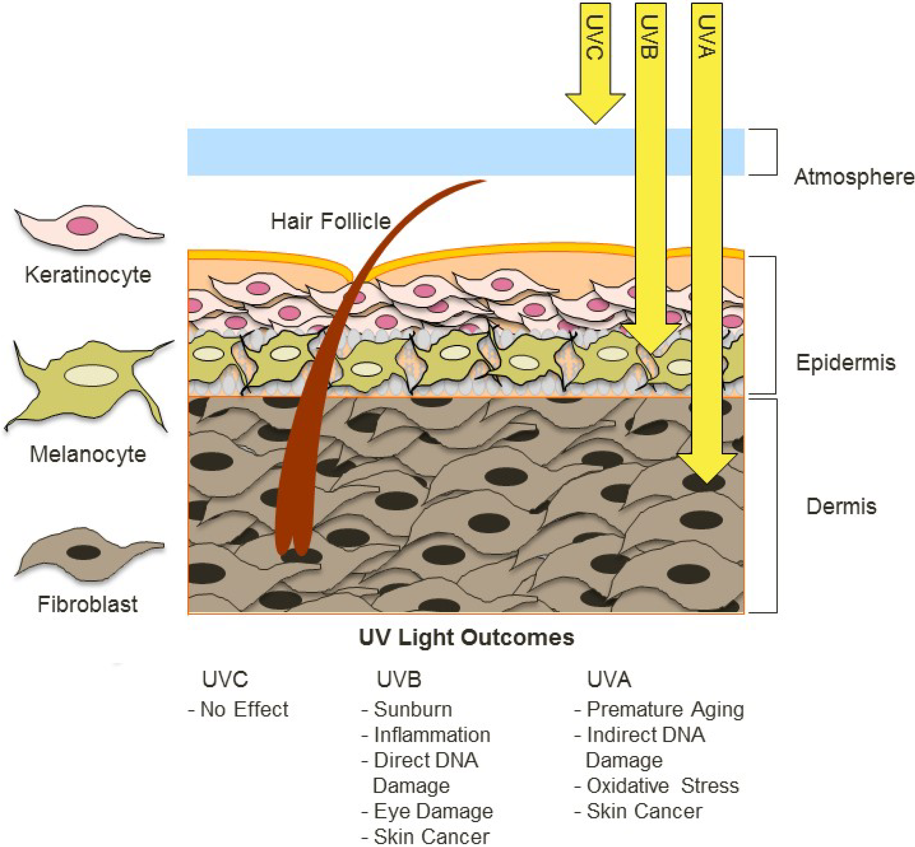
UV radiation is common to many envrioments and it varies in widely in its intensity and composition, such as differing ratios of UV-A and UV-B radiation. The different forms of UV radaition have distinct, and frequently harmful effects on organisms and biological systems. For example, the following diagram depicts the effects of different forms of UV radiation on the skin.
UV radiation is considered an important environmental stressor that organisms need to defend against. There are three primary methods for defending against UV radiation:
- Avoidance
- Photoprotection
- Repair
Since the red flour beetle (Tribolium castaneum) spends much of its life cycle in infested grains, the larvae does not typically experience high levels of UVR. Furthermore, the larvae of the red flour beetle is light in pigmentation and does not appear to employ photoprotective pigments (e.g., melanin) to defend against harmful levels of UV radiation (UVR).
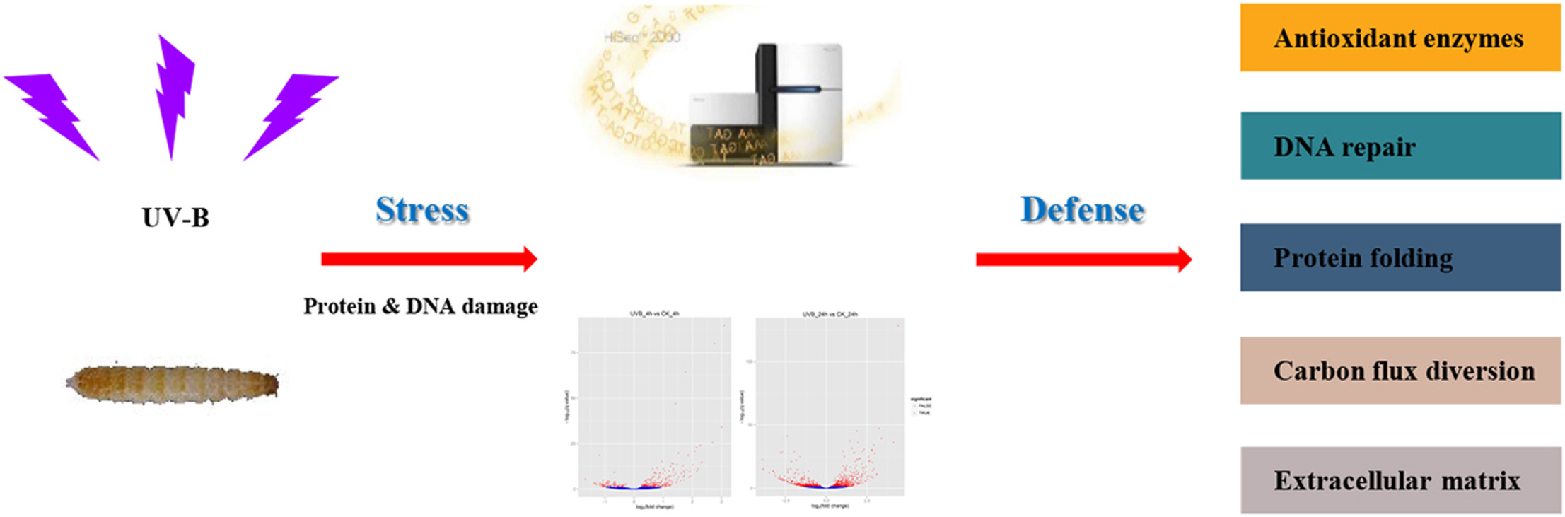
So, how do the larvae handle any exposure to UV radiation? In their study, the authors investigate the defense strategy against UV-B radiation in the red flour beetle. The following graphical abstract illustrates the design of their study, and how the omics data that we will be using in this workshop was collected.
What is Gene Transcription?
Before we proceed with our bioinformatics analysis we should consider the data that we will be working with, and how it is collected. In this workshop we will be using several different file types for the various biological data that we will need in the bioinformatics analysis workflow. Remember that omics technologies include genetic, transcriptomic, proteomic, and metabolomic data.
First, we will need to use transcription sequence data. Transcription is the first step in gene expression, which involves copying the DNA sequence of a gene to make a RNA molecule. For a protein-coding gene, the RNA copy (transcript) carries the information needed to build a polypeptide (protein or protein subunit).
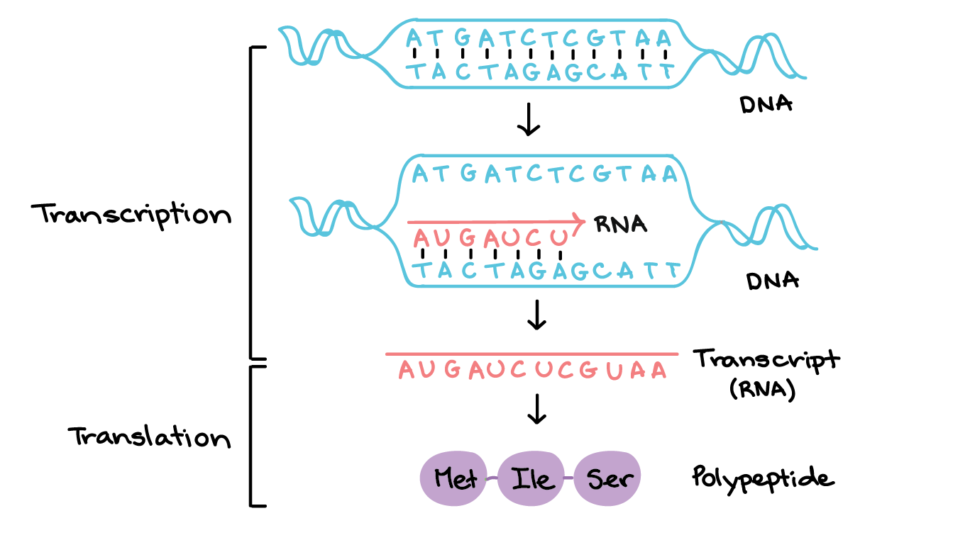
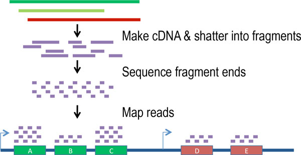
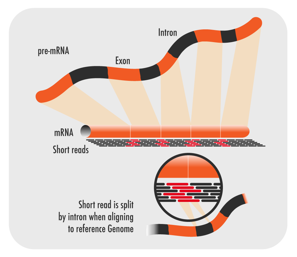
The transcription of genes can be measured using next-generation sequencing techniques that produces millions of sequences (reads) in a short time. This process depicted in the following schematic representation of a RNA sequencing protocol.
Transcription can provide whole genome-wide RNA expression profiles, and is useful for identifying key factors influencing transcription in different environmental conditions. For example, consider the following plot of transcription sequence coverage for a gene model (green) in a species of Daphnia, which has been subjected to a control of visible light (blue) and treatment of UV radiation (red).
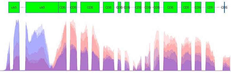
As we can see, the coding sequences (CDS) of the predicted gene model are more highlighy expressed in the tratment of UV radiation. This is visible by the red peaks of transcription sequence read coverage, which are showing the higher frequency of sequence reads from the UV treatment matching up (mapping) to the CDS than the visible light sequences.
Transcriptomic Data Collection
There are several pieces of transcriptomic data that we will need to collect before we can proceed with the bioinformatics analysis. Transcription data are essentially strings of characters in files with very specific formatting.
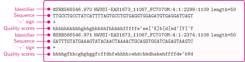
In this workshop we will be using transcription sequence data in the FASTQ format. This format stores both biological sequences and their corresponding quality scores. Each sequence typically has the following four lines of information.
- A line beginning with @ followed by a sequence identifier and optional description (comment)
- The raw sequence letters
- A line beginning with +, sometimes followed by the same comment as the first line
- A line encoding the quality values for the sequence in line 2, with the same numbers of symbols as letters in the sequence
Software Prerequisite
Note: Make sure that the SRA Toolkit is installed before we proceed to download the transcriptomic data we need. To download the SRA toolkit:
- navigate to the installation instructions
- find the appropriate instructions for your operating system (OS)
Further information and tips for installing the SRA toolkit may be found on the Setup page.
The SRA Toolkit allows you to retrieve data from the SRA for a specific research project using the associated accession number. Additionally, it allows you to produce data file formats like FASTQ using fastq-dump, which is one of the command line tools packaged in the SRA Toolkit.
With the SRA Toolkit installed, we can proceed with collecting the transcriptomic data we need for our bioinformatics analysis. Remeber that we are following the example of the study performed by the authors of “Digital gene expression profiling in larvae of Tribolium castaneum at different periods post UV-B exposure”.
Coding Challenge - Transcriptomic Data Collection
Scripting & Pipelining Tip!
The primary benefit of scripting is the ability to save modular pieces of code to re-use later. As a first step to designing a pipeline, it is a good idea to work through a simple example using data. While you are working through the exercises in this workshop, make sure to store the pieces of code that you write to perform each task.
Recall that the file extension for BASH scripts is .sh.
Note: it is highly recommended that you also write a comment for each piece of code that states why you are using that piece of code. Also, you may wish to leave a comment about the purpose, or what that piece of code does.
Let’s find the transcriptomic data we need by navigating the internet. This data may be accessed by:
Step 1
Go to the paper on the publisher’s website, and be sure you have access to the full article. Recall, “Digital gene expression profiling in larvae of Tribolium castaneum at different periods post UV-B exposure”.
Tip! - Task 1
A simple way to gain access to a specific publication is by searching the name of a paper using the Hesburgh Library website
Step 2
Search the paper for the SRA “accession” number associated with the study.
Tip! - Task 2
Search the paper for “accession” (Mac: command+f, Windows: cntrl+f) and copy the Accession No.
Solution - Task 2
The Accession No. is PRJNA504739 for the transcriptomic data.
Step 3
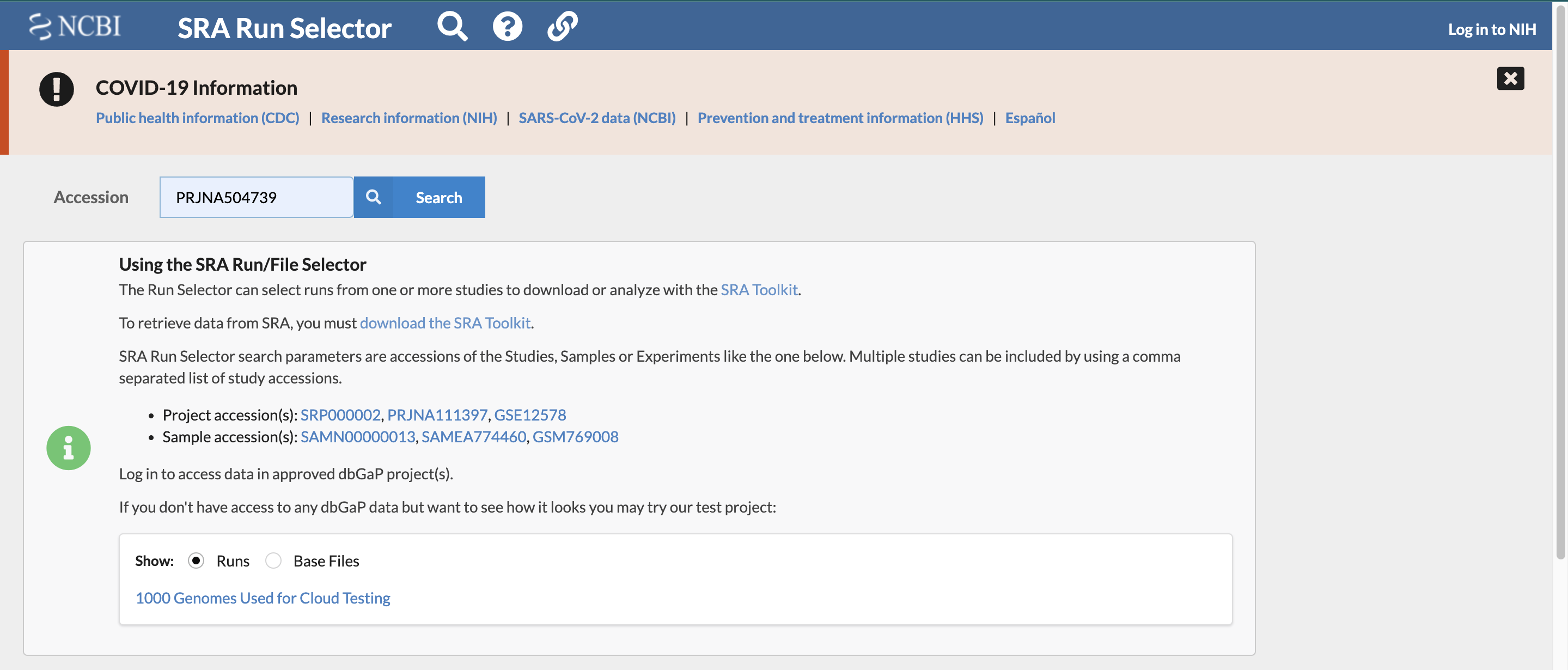
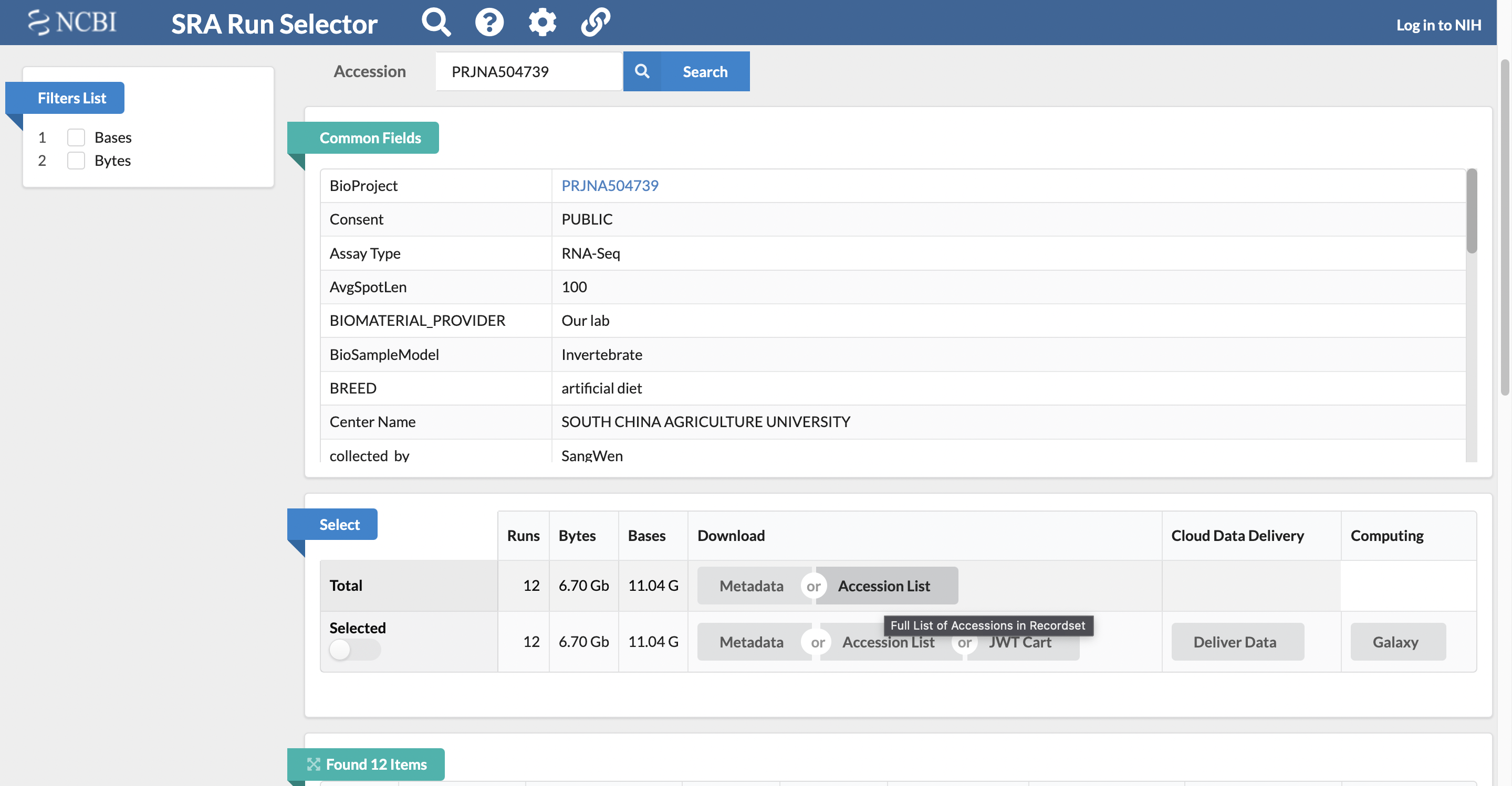
Find the list of accession numbers for the set of transcriptomic data associated with the study by searching for the previously found study accession number using the “SRA Run Selector” on the NCBI website. It is here you will find futher information about each of the sample files as well.
Solution - Task 3
To find the list of accession numbers for the transcripts:
- enter the accession number you found in the paper in the search box as follows:
Step 4
Retrieve the total accession list for the study, which has the SRA accession numbers for all of the samples.
Solution - Task 4
It is possible to download the full list of SRA accession numbers for all the samples associated with the study by selecting to download the total accession list from the “Select” section of the page.
Step 5
Retrieve the all of the transcriptomic sequence data for the study using the SRA accession numbers for all of the samples.
Scripting & Pipelining Tip!
Remember to save these pieces of code in files with the .sh extension While you are working through these exercises!
Solution - Task 5
To retrieve the full set of samples, use the following prefetch and fastq-dump commands and accession numbers. This will take several moments.
prefetch SRR8288561 SRR8288562 SRR8288563 SRR8288564 SRR8288557 SRR8288560 SRR8288558 SRR8288559 SRR8288565 SRR8288566 SRR8288567 SRR8288568
fastq-dump --gzip SRR8288561; fastq-dump --gzip SRR8288562; fastq-dump --gzip SRR8288563; fastq-dump --gzip SRR8288564; fastq-dump --gzip SRR8288557; fastq-dump --gzip SRR8288560
fastq-dump --gzip SRR8288558; fastq-dump --gzip SRR8288559; fastq-dump --gzip SRR8288565; fastq-dump --gzip SRR8288566; fastq-dump --gzip SRR8288567; fastq-dump --gzip SRR8288568
Tip!
Note: that if a terminal command is taking a long time to run, you may use the Cntrl + C keyboard shortcut to kill it and force it to stop running.
Transcriptomic Data Quality Control
An important part of any bioinformatics analysis workflow is the assesment and quality control of your data. In this workshop we are using RNA sequencing reads, which may need to be cleaned if they are raw and include extra pieces of unnecessary data (e.g., adapter sequences.
Software Prerequisites
Note: be sure that you have installed the FastQC software program before we proceed with the bioinformatics analysis workflow.
Further information and tips for installing the FastQC software may be found on the Setup page.
To check if the transcriptomic data that we downloaded has been cleaned already, we need to use the FastQC bioinformatics software tool.
Coding Challenge
Let’s use the following fastqc command to view the quality of one of the sequence read data sets.
fastqc SRR8288561.fastq.gz --extractBe aware that you can also use the FastQC application to view the quality of transcript data using a user interface.
Now we can compare the results that we recieved from the analysis of this sample to the docummentation for FastQC, which include a “Good Illumina Data” example and a “Bad Illumina Data” example.
Genomic Data Collection
Next, we need to collect the neccessary genomic data. Where you get your genomic data may depend on several factors. For example, some or all of the data that you need may be available through an online database.
Checklist
These are common online databases for bioinformatics analysis:
- Database of Genomic Structural Variation (dbVar) – insertions, deletions, duplications, inversions, mobile element insertions, translocations, and complex chromosomal rearrangements
- Database of Genotypes and Phenotypes(dbGaP) - developed to archive and distribute the data and results from studies that have investigated the interaction of genotype and phenotype in Humans
- Database of Single Nucleotide Polymorphisms (dbSNP) - multiple small-scale variations that include insertions/deletions, microsatellites, and non-polymorphic variants
- GenBank - the NIH genetic sequence database, an annotated collection of all publicly available DNA sequences
- Gene - integrates nomenclature, Reference Sequences (RefSeqs), maps, pathways, variations, phenotypes, and links to genome-, phenotype-, and locus-specific from a wide range of species
- Gene Expression Omnibus (GEO) - a public functional genomics data repository supporting MIAME-compliant data submissions
- Gene Expression Omnibus Datasets - stores curated gene expression DataSets, as well as original Series and Platform records in the Gene Expression Omnibus (GEO) repository
- Genome Data Viewer (GDV) - a genome browser supporting the exploration and analysis of more than 380 eukaryotic RefSeq genome assemblies
- International Genome Sample Resource (IGSR) - from the 1000 Genomes Project that ran between 2008 and 2015, which created the largest public catalogue of human variation and genotype data
- The Reference Sequence (RefSeq) - a collection that provides a comprehensive, integrated, non-redundant, well-annotated set of sequences, including genomic DNA, transcripts, and proteins
Depedning on the organisms that you are working with, you may need to locate data in more organism specific databases. We are working with data for the Tribolium castaneum (red flour beetle), which is an arthropod in the order Coleoptera and family Tenebrionidae. So, we are also interested in accessing data from InsectBase. Specifically, we will need:
- reference genome
- genomic features
Challenge
Navigate to the Tribolium castaneum organism page of the InsectBase website and under the “Download” section of the page:
- click the red word Genome
- click the blue word GFF3
This will automatically begin downloading each of the necessary genomic data files.
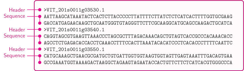
The reference genome is in the FASTA file format, and has the .fa file extension. This format is commonly used when storing DNA sequence data.
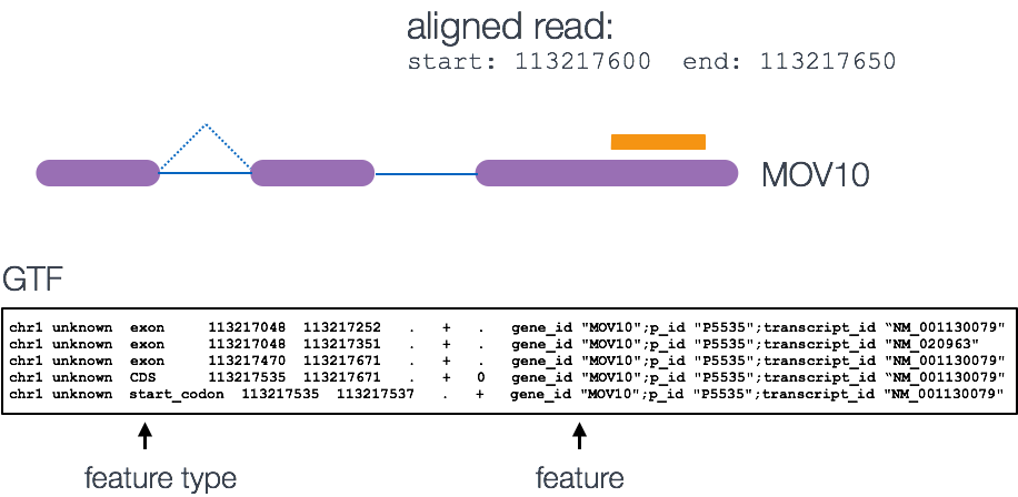
The genomic features file is in the GFF3 file format, and has the .gff3 file extension. This format is a tab-delimited text file that describes the information about any feature of a nucleic acid or protein sequence. These features may include anything from coding sequences (CDS), microRNAs, binding domains, open reading frames (ORFs), etc.
Checklist
GFF3 has 9 required fields, though not all are utilized (either blank or a default value of .):
- Sequence ID - a string with the ID of the sequence
- Source - describes the algorithm or the procedure that generated this feature
- Feature Type - describes what the feature is (mRNA, domain, exon, etc.)
- Feature Start - starting position for the feature
- Feature End - ending position for the feature
- Score - typically E-values for sequence similarity and P-values for predictions
- Strand - a single character that indicates the strand of the feature
- Phase - indicates where the feature begins with reference to the reading frame
- Atributes - a semicolon-separated list of tag-value pairs, providing additional information about each feature
Omics Data Preparation - Command Line
Now that we have the necessary transcript and genomic data, we can begin the process of preparing our data for statistical analysis. This will require proceeding through several steps of the bioinformatics workflow. Recall:
- data collection - SRA toolkit
- quality control - fastqc
- data preparation
- convert genomic data format - gffread
- align transcriptomic data - hisat2
- quantify transcript alignments - featureCounts
- basic statistical analysis and visualization (exact tests) - edgeR
- advanced statistical analysis and visualization (generalized linear models) - edgeR
Software Prerequisites
Note: be sure that you have installed the following software before we proceed with the bioinformatics analysis workflow.
Further information and tips for installing the fastqc, gffread, and hisat2 software programs may be found on the Setup page.
Convert Genomic Data Format
The first step in our bioinformatics workflow is to convert one of the genomic data files to the format expected by our downstread analysis tools. The genome features file that we downloaded from InsectBase for Tribolium castaneum is in the gff3 format, but it needs to be in gtf format to use with Hisat2. This is because there are some important formatting differences between the two genomic feature file types.
Coding Challenge
Let’s use the gffread command line tool to convert the genomic features file from gff3 to gtf format. Hint: check out the manual page for gffread to learn more about the different options.
gffread -E -F -T Tribolium_castaneum.gff3 -o Tribolium.gtf
Align Transcriptomic Data
Next, we need to prepare the transcriptomic sequence data files for statistical analysis by aligning the reads to the reference genome. Recall that our RNA sequence analysis workflow involves mapping the shattered reads to a reference genome.
Coding Challenge
Let’s use the Hisat2 command line tool to map the transcriptomic sequence reads to the reference genome of Tribolium castaneum. This is done in two steps. Hint: check out the manual page for Hisat2 to learn more about the different options.
Step 1
First, we need to build a HISAT2 index from the set of DNA sequences for Tribolium castaneum contained in the reference genome fasta file. The build files that are produced by running the following command are needed to map the aligned reads to the reference using the hisat2 commands in the next step (Step 2).
hisat2-build Tribolium_castaneum.genome.fa TriboliumBuildStep 2
Second, we can use the hisat2 command to map each read to the reference genome. This results in an output sam file for each of the input compressed transcript sequence fastq.gz files.
hisat2 -q -x TriboliumBuild -U SRR8288561.fastq.gz -S SRR8288561_accepted_hits.sam
hisat2 -q -x TriboliumBuild -U SRR8288562.fastq.gz -S SRR8288562_accepted_hits.sam
hisat2 -q -x TriboliumBuild -U SRR8288563.fastq.gz -S SRR8288563_accepted_hits.sam
hisat2 -q -x TriboliumBuild -U SRR8288564.fastq.gz -S SRR8288564_accepted_hits.sam
hisat2 -q -x TriboliumBuild -U SRR8288557.fastq.gz -S SRR8288557_accepted_hits.sam
hisat2 -q -x TriboliumBuild -U SRR8288560.fastq.gz -S SRR8288560_accepted_hits.sam
hisat2 -q -x TriboliumBuild -U SRR8288558.fastq.gz -S SRR8288560_accepted_hits.sam
hisat2 -q -x TriboliumBuild -U SRR8288567.fastq.gz -S SRR8288560_accepted_hits.sam
hisat2 -q -x TriboliumBuild -U SRR8288568.fastq.gz -S SRR8288560_accepted_hits.sam
hisat2 -q -x TriboliumBuild -U SRR8288559.fastq.gz -S SRR8288560_accepted_hits.sam
hisat2 -q -x TriboliumBuild -U SRR8288565.fastq.gz -S SRR8288560_accepted_hits.sam
hisat2 -q -x TriboliumBuild -U SRR8288566.fastq.gz -S SRR8288560_accepted_hits.sam
Omics Data Preparation - R
Now that we have the transcript sequence reads aligned to the reference genome, we can begin to quantify the number of reads that map to each genomic feature from the features file. Recall that we are able to count the number of reads that map to each feature in a genome to compare the effects of a treatment, such as UV radiation exposure.
Scripting & Pipelining Tip!
Remember that the primary benefit of scripting is the ability to save modular pieces of code to re-use later. As a first step to designing a pipeline, it is a good idea to work through a simple example using data. While you are working through the exercises in this workshop, make sure to store the pieces of code that you write to perform each task.
After going through your bioinformatics workflow with a simple data example to make an initial scripting pipeline, it is helpful to test your pipeline with a more complicated example. This will allow you to identify the pieces of your pipeline that may easily be generalized for future analysis. For example, defining your script to allow users to enter names for the files they wish to process when they run the script.
Recall that the file extension for R scripts is .r or .R.
Note: it is highly recommended that you also write a comment for each piece of code that states why you are using that piece of code. Also, you may wish to leave a comment about the purpose, or what that piece of code does.
Coding Challenge
Software Prerequisites
Note: be sure that you have loaded the [Rsubread][rsubreadCite] R library before we proceed with the bioinformatics analysis workflow.
Further information and tips for installing the Rsubread R library may be found on the Setup page.
The featureCounts function of the Rsubread library allows us to count the number of transcripts that map to each genomic feature in the Tribolum castaneum reference genome.
Note: the ? symbol can be prepended (e.g., ?featurecounts) to most function names in R to retrieve more information about the function.
Tip!
To make the process easier, remember to set your working directory before proceeding with any coding in R.
setwd("/YOUR/WORKSHOP/DIRECTORY/PATH")Also, remember to load the Rsubread library before you attempt to use the featureCounts function.
library("Rsubread")
As a first step, we need to quantify (count) the number of transcript sequence reads that have mapped (aligned) to the features of the Tribolium castaneum genome.
So to quantify the read fragments that map to the genomic features of the red flour beetle genome, we will use the fetureCounts function with the output Hisat2 sam files from the previous step of the bioinformatics workflow.
# control samples at 4h
cntrl1_fc <- featureCounts(files="SRR8288561_accepted_hits.sam", annot.ext="Tribolium.gtf", isGTFAnnotationFile=TRUE)
cntrl2_fc <- featureCounts(files="SRR8288562_accepted_hits.sam", annot.ext="Tribolium.gtf", isGTFAnnotationFile=TRUE)
cntrl3_fc <- featureCounts(files="SRR8288563_accepted_hits.sam", annot.ext="Tribolium.gtf", isGTFAnnotationFile=TRUE)

# control samples 24h
cntrl1_fc_24h <- featureCounts(files="SRR8288558_accepted_hits.sam", annot.ext="Tribolium.gtf", isGTFAnnotationFile=TRUE)
cntrl2_fc_24h <- featureCounts(files="SRR8288567_accepted_hits.sam", annot.ext="Tribolium.gtf", isGTFAnnotationFile=TRUE)
cntrl3_fc_24h <- featureCounts(files="SRR8288568_accepted_hits.sam", annot.ext="Tribolium.gtf", isGTFAnnotationFile=TRUE)

# treatment samples at 4h
treat1_fc <- featureCounts(files="SRR8288564_accepted_hits.sam", annot.ext="Tribolium.gtf", isGTFAnnotationFile=TRUE)
treat2_fc <- featureCounts(files="SRR8288557_accepted_hits.sam", annot.ext="Tribolium.gtf", isGTFAnnotationFile=TRUE)
treat3_fc <- featureCounts(files="SRR8288560_accepted_hits.sam", annot.ext="Tribolium.gtf", isGTFAnnotationFile=TRUE)

# treatment samples 24h
treat1_fc_24h <- featureCounts(files="SRR8288559_accepted_hits.sam", annot.ext="Tribolium.gtf", isGTFAnnotationFile=TRUE)
treat2_fc_24h <- featureCounts(files="SRR8288565_accepted_hits.sam", annot.ext="Tribolium.gtf", isGTFAnnotationFile=TRUE)
treat3_fc_24h <- featureCounts(files="SRR8288566_accepted_hits.sam", annot.ext="Tribolium.gtf", isGTFAnnotationFile=TRUE)
Tip!
Checkout what the resulting data frames looks like using the names and head commands. For example:
names(cntrl1_fc)

head(cntrl1_fc$counts)
Before we can move on to any statistical analysis, we need to prepare the data by adding all of the results to a single data frame.
# prepare data frame of sequence read count data
tribolium_counts <- data.frame(
  SRR8288561 = unname(cntrl1_fc_4h$counts),
  SRR8288562 = unname(cntrl2_fc_4h$counts),
  SRR8288563 = unname(cntrl3_fc_4h$counts),
  SRR8288558 = unname(cntrl1_fc_24h$counts),
  SRR8288567 = unname(cntrl2_fc_24h$counts),
  SRR8288568 = unname(cntrl3_fc_24h$counts),
  SRR8288564 = unname(treat1_fc_4h$counts),
  SRR8288557 = unname(treat2_fc_4h$counts),
  SRR8288560 = unname(treat3_fc_4h$counts),
  SRR8288559 = unname(treat1_fc_24h$counts),
  SRR8288565 = unname(treat2_fc_24h$counts),
  SRR8288566 = unname(treat3_fc_24h$counts)
)

# checkout what the resulting counts data frame looks like
head(tribolium_counts)

# set the row names of the counts data frame using a featureCounts results data frame
rownames(tribolium_counts) <- rownames(cntrl1_fc$counts)

# checkout what the updated counts data frame looks like
head(tribolium_counts)
Scripts for this Lesson
Here is the BASH script with the code from this lesson.
Key Points
Explore available omics databases before you design your analysis workflow
Thoroughly explore the supplamental materials of research study papers.
Make sure to install any necessry software in advance.
Always include informative documents for your data.
Carefully name and store your raw and calculated data files.